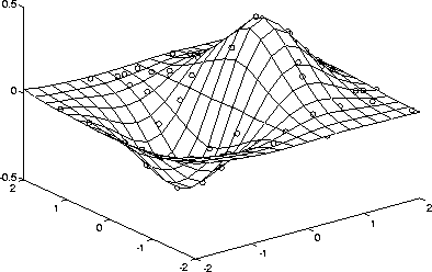
mesh(XI,YI,ZI), hold
plot3(x,y,z,'o'), hold off
| MATLAB Functions | Help Desk |
griddata
Data gridding
ZI = griddata(x,y,z,XI,YI)
[XI,YI,ZI] = griddata(x,y,z,xi,yi)
[...] = griddata(...,method)
ZI = griddata(x,y,z,XI,YI)
fits a surface of the form z = f(x,y) to the data in the (usually) nonuniformly spaced vectors (x,y,z). griddata interpolates this surface at the points specified by (XI,YI) to produce ZI. The surface always passes through the data points. XI and YI usually form a uniform grid (as produced by meshgrid).
XI can be a row vector, in which case it specifies a matrix with constant columns. Similarly, YI can be a column vector, and it specifies a matrix with constant rows.
[XI,YI,ZI] = griddata(x,y,z,xi,yi)
returns the interpolated matrix ZI as above, and also returns the matrices XI and YI formed from row vector xi and column vector yi. These latter are the same as the matrices returned by meshgrid.
[...] = griddata(...,method)
uses the specified interpolation method:method defines the type of surface fit to the data. The 'cubic' and 'invdist' methods produce smooth surfaces while 'linear' and 'nearest' have discontinuities in the first and zero'th derivatives, respectively. All the methods except 'invdist' are based on a Delaunay triangulation of the data.
XI and YI can be matrices, in which case griddata returns the values for the corresponding points (XI(i,j),YI(i,j)). Alternatively, you can pass in the row and column vectors xi and yi, respectively. In this case, griddata interprets these vectors as if they were matrices produced by the commandmeshgrid(xi,yi).
The griddata(...,'invdist') command uses the inverse distance method of [1]. The other methods are based on Delaunay triangulation (see delaunay).
Sample a function at 100 random points between ±2.0:
rand('seed',0)
x = rand(100,1)*4-2; y = rand(100,1)*4-2;
z = x.*exp(-x.^2-y.^2);
x, y, and z are now vectors containing nonuniformly sampled data. Define a regular grid, and grid the data to it:
Plot the gridded data along with the nonuniform data points used to generate it:ti=-2:.25:2;[XI,YI]=meshgrid(ti,ti);ZI=griddata(x,y,z,XI,YI);
mesh(XI,YI,ZI), holdplot3(x,y,z,'o'), holdoff

delaunay, interp2, meshgrid
[1] Sandwell, David T., "Biharmonic Spline Interpolation of GEOS-3 and SEASAT Altimeter Data", Geophysical Research Letters, 2, 139-142,1987.
[2] Watson, David E., Contouring: A Guide to the Analysis and Display of Spatial Data, Tarrytown, NY: Pergamon (Elsevier Science, Inc.): 1992.