| Getting Started with MATLAB | Help Desk |
Handle Graphics
MATLAB provides a set of low-level functions that allows you to create and manipulate lines, surfaces, and other graphics objects. This system is called Handle Graphics®. Graphics objects are the basic drawing primitives of MATLAB's Handle Graphics system. The objects are organized in a tree structured hierarchy. This reflects the interdependence of the graphics objects. For example, Line objects require Axes objects as a frame of reference. In turn, Axes objects exist only within Figure objects. There are eleven kinds of Handle Graphics objects:A is the Dürer magic square, then
h = plot(A)creates a line plot with four lines, one for each column of
A. It also returns a vector of handles such as
h =
   9.00024414062500
   6.00048828125000
   7.00036621093750
   8.00036621093750
The actual numerical values are irrelevant and may vary from system to system. Whatever the numbers are, the important fact is that
h(1) is the handle for the first line in the plot, h(2) is the handle for the second, and so on.
MATLAB provides several functions to access frequently used object handles:
gcf
gca
gco
delete function, passing the object's handle as an argument. For example, delete the current axes (and all of its children) with the statement:
delete(gca)Calling the function named after any object creates one of those objects. For example, the
text function creates text objects, the figure function creates figure objects, and so on. MATLAB's high-level graphics functions (like plot and surf) call the appropriate low-level function to draw their respective graphics.
Low-level functions simply create one of the eleven graphics objects defined by MATLAB with the exception of the root object, which only MATLAB can create. For example:
line([1 3 6], [8 -2 0], 'Color', 'red')All objects have properties that control how they are displayed. MATLAB provides two mechanisms for setting the values of properties. Object properties can be set by the object creation function, or can be changed with the
set function after the object already exists. For example, these statements create three objects and override some of their default properties.
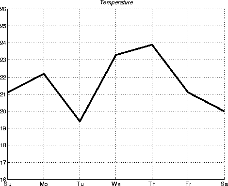
days = ['Su';'Mo';'Tu';'We';'Th';'Fr';'Sa']
temp = [21.1 22.2 19.4 23.3 23.9 21.1 20.0];
f = figure
a = axes('YLim',[16 26],'Xtick',1:7,'XTickLabel',days)
h = line(1:7,temp)

days is a character array containing abbreviations for the days of the week and temp is a numeric array of typical temperatures. The figure window is created by calling figure with no arguments, so it has the default properties. The axes exists within the figure and has a specified range for the scaling of the y-axis and specified labels for the tick marks on the x-axis. The line exists within the axes and has specified values for the x and y data. The three object handles f, a, and h, are saved for later use.
Object properties are specified by referencing the object after its creation. To do this, use the handle returned by the creating function.
The set function allows you to set any object's property by specifying the object's handle and any number of property name/property value pairs. For instance, to change the color and width of the line from the previous example,
set(h,'Color',[0 .8 .8],'LineWidth',3)To see a list of all settable properties for a particular object, call
set with the object's handle:
set(h)

    Color
    EraseMode: [ {normal} | background | xor | none ]
    LineStyle: [ {-} | -- | : | -. | none ]
    LineWidth
    Marker:
    MarkerSize
    ...
    XData
    YData
    ZData
To see a list of all current settings properties for a particular object, call get with the object's handles:
get(h)

    Color = [0 0.8 0.8]
    EraseMode = normal
    LineStyle =
    LineWidth = [3]
    Marker = none
    MarkerSize = [6]
    ...
    XData = [ (1 by 7) double array]
    YData = [ (1 by 7) double array]
    ZData = []
To query the value of a property, use get with the property name:
get(h,'Color')

ans =

     0     0.8000 0.8000
The axes object carries many of the detailed properties of the overall graphic. For example, the title is another child of the axes. The statements:
t = get(a,'title');
set(t,'String','Temperature','FontAngle','oblique')
specify a particular title. The
title function provides another interface to the same properties.
Here is a simple example illustrating how to use Handle Graphics to build user interfaces. The statement
b = uicontrol('Style','pushbutton', ...
      'Units','normalized', ...
      'Position',[.5 .5 .2 .1], ...
      'String','click here');
creates a pushbutton in the center of a figure window and returns a handle to the new object. But, so far, clicking on the button does nothing. The statement
s = 'set(b,''Position'',[.8*rand .9*rand .2 .1])';creates a string containing a command that alters the pushbutton's position. Repeated execution of
eval(s)moves the button to random positions. Finally,
set(b,'Callback',s)installs
s as the button's callback action, so every time you click on the button, it moves to a new position.
MATLAB provides several ways of generating moving, animated, graphics. Using the EraseMode property is appropriate for long sequences of simple plots where the change from frame to frame is minimal. Here is an example showing simulated Brownian motion. Specify a number of points, like
n = 20and a temperature or velocity, such as
s = .02The best values for these two parameters depend upon the speed of your particular computer. Generate
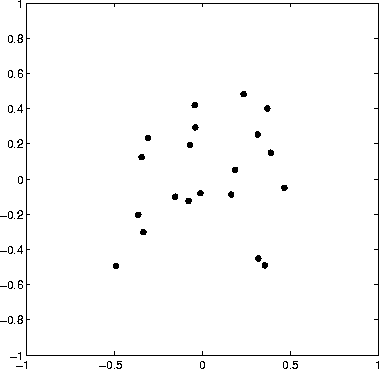
n random points with (x,y) coordinates between -1/2 and +1/2
x = rand(n,1)-0.5;
y = rand(n,1)-0.5;
Plot the points in a square with sides at -1 and +1. Save the handle for the vector of points and set its
EraseMode to xor. This tells the MATLAB graphics system not to redraw the entire plot when the coordinates of one point are changed, but to restore the background color in the vicinity of the point using an "exclusive or" operation.
h = plot(x,y,'.');
axis([-1 1 -1 1])
axis square
grid off
set(h,'EraseMode','xor','MarkerSize',18)
Now begin the animation. Here is an infinite
while loop, which you will eventually break out of by typing <ctrl>-c. Each time through the loop, add a small amount of normally distributed random noise to the coordinates of the points. Then, instead of creating an entirely new plot, simply change the XData and YData properties of the original plot.
while 1
   x = x + s*randn(n,1);
   y = y + s*randn(n,1);
   set(h,'XData',x,'YData',y)
end
How long does it take for one of the points to get outside of the square? How long before all of the points are outside the square?
 If you increase the number of points in the Brownian motion example to something like
 n = 300, the motion is no longer very fluid; it takes too much time to draw each time step. It becomes more effective to save a predetermined number of frames as bitmaps and to play them back as a movie.
First, decide on the number of frames, say
nframes = 50Next, set up the first plot as before, except do not use
EraseMode.
x = rand(n,1)-0.5;
y = rand(n,1)-0.5;
h = plot(x,y,'.')
set(h,'MarkerSize',18)
axis([-1 1 -1 1])
axis square
grid off
Now, allocate enough memory to save the complete movie,
M = moviein(nframes)This sets aside a large matrix with
nframes columns. Each column is long enough to save one frame. The total amount of memory required is proportional to the number of frames, and to the area of the current axes; it is independent of the complexity of the particular plot. For 50 frames and the default axes, over 7.5 megabytes of memory is required. This example is using square axes, which is slightly smaller, so only about 6 megabytes is required.
Generate the movie and use getframe to capture each frame.
for k = 1:nframes
   x = x + s*randn(n,1);
   y = y + s*randn(n,1);
   set(h,'XData',x,'YData',y)
   M(:,k) = getframe;
end
Finally, play the movie 30 times.
movie(30)